Note
Go to the end to download the full example code.
Digit Classification with SomClassifier
Classifies handwritten digits from the sklearn digits dataset using
SomClassifier wrapped in a scikit-learn Pipeline with StandardScaler.
The dataset contains 1 797 grayscale images (8×8 pixels, 64 features) of digits 0–9.
Build and Train Pipeline
SomClassifier is a drop-in replacement for any scikit-learn classifier.
Wrapping it in a Pipeline applies StandardScaler automatically
during both fit and predict.
from sklearn.datasets import load_digits
from sklearn.pipeline import Pipeline
from sklearn.preprocessing import StandardScaler

from dbgsom.SomClassifier import SomClassifier

digits_X, digits_y = load_digits(return_X_y=True)

som = SomClassifier(
    lambda_=76.6,
    n_iter=500,
    sigma_end=0.5,
    random_state=42,
    tau_2=0.01,
)

pipe = Pipeline(steps=[("scaler", StandardScaler()), ("som", som)])
pipe.fit(digits_X, digits_y)
Pipeline(steps=[('scaler', StandardScaler()),
                ('som',
                 SomClassifier(lambda_=76.6, random_state=42, sigma_end=0.5,
                               tau_2=0.01))])
In a Jupyter environment, please rerun this cell to show the HTML representation or trust the notebook. On GitHub, the HTML representation is unable to render, please try loading this page with nbviewer.org.
Parameters
Fitted attributes
Parameters
Fitted attributes
64 features
| x0 |
| x1 |
| x2 |
| x3 |
| x4 |
| x5 |
| x6 |
| x7 |
| x8 |
| x9 |
| x10 |
| x11 |
| x12 |
| x13 |
| x14 |
| x15 |
| x16 |
| x17 |
| x18 |
| x19 |
| x20 |
| x21 |
| x22 |
| x23 |
| x24 |
| x25 |
| x26 |
| x27 |
| x28 |
| x29 |
| x30 |
| x31 |
| x32 |
| x33 |
| x34 |
| x35 |
| x36 |
| x37 |
| x38 |
| x39 |
| x40 |
| x41 |
| x42 |
| x43 |
| x44 |
| x45 |
| x46 |
| x47 |
| x48 |
| x49 |
| x50 |
| x51 |
| x52 |
| x53 |
| x54 |
| x55 |
| x56 |
| x57 |
| x58 |
| x59 |
| x60 |
| x61 |
| x62 |
| x63 |
Parameters
| lambda_ | 76.6 | |
| sigma_end | 0.5 | |
| random_state | 42 | |
| tau_2 | 0.01 | |
| n_iter | 500 | |
| sigma_start | None | |
| sigma_fine | None | |
| vertical_growth | False | |
| decay_function | 'exponential' | |
| neighborhood_function | 'gaussian' | |
| neighborhood_cutoff | 3.0 | |
| verbose | False | |
| coarse_training_frac | 0.5 | |
| convergence_threshold | 0.001 | |
| max_neurons | None | |
| metric | 'euclidean' | |
| growth_criterion | 'quantization_error' | |
| min_samples_vertical_growth | 100 | |
| n_jobs | 1 | |
| winner_stability_threshold | 0.01 | |
| pointer_search | 'fine' | |
| cutgauss_phase | 'fine' | |
| smoothing_steps | 0 | |
| smoothing_epsilon | 0.5 |
Fitted attributes
| Name | Type | Value |
|---|---|---|
| classes_ | ndarray[int64](10,) | [0,1,2,...,7,8,9] |
| converged_ | bool | True |
| growing_threshold_ | float | 598.4 |
| lambda_ | float | 76.6 |
| n_features_in_ | int | 64 |
| n_iter_ | int | 91 |
| neurons_ | list | [(0, 0), (0, 1), (1, 0), (1, 1), ...] |
| qe_0_ | float | 1.308e+04 |
| quantization_error_ | float | 5.061 |
| random_state_ | RandomState | RandomState(M...0x71906D6A9840 |
| som_ | Graph | <networkx.cla...x71906d6b7380> |
| topographic_error_ | float | 0.1302 |
| topographic_product_ | float | -0.04101 |
| weights_ | ndarray[float64](30, 64) | [[ 0. ,-0.34,-1.08,..., 0.8 ,-0.04,-0.19], [ 0. ,-0.32,-0.64,..., 1.05, 1.17, 0.57], [ 0. ,-0.02,-0.08,..., 0.08, 0.36, 0.57], ..., [ 0. ,-0.33,-0.27,...,-0.29,-0.43,-0.2 ], [ 0. ,-0.3 ,-0.62,...,-1.12,-0.51,-0.2 ], [ 0. ,-0.34,-0.58,...,-1.07,-0.51,-0.2 ]] |
Evaluation
Print accuracy and topographic quality metrics.
print(f"Accuracy:           {pipe.score(digits_X, digits_y):.4f}")
print(f"Topographic error:  {som.topographic_error_:.4f}")
print(f"Quantization error: {som.quantization_error_:.4f}")
Accuracy:           0.8625
Topographic error:  0.1302
Quantization error: 5.0607
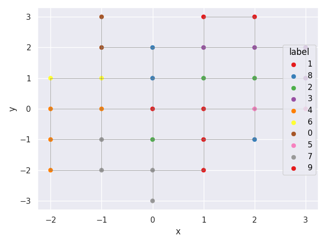
Grid Layout – Neurons by Dominant Class
Each neuron colored by its dominant digit class. Spatial clustering shows how the SOM organizes the digit space.
som.plot(layout="grid", color="label", palette="Set1").show()
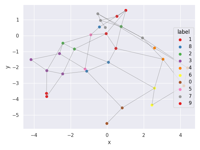
PCA Layout
Same coloring but neurons arranged by PCA of their weight vectors. Reveals the structure of the learned representation in weight space.
som.plot(layout="pca", color="label", palette="Set1", X=digits_X).show()
Total running time of the script: (0 minutes 12.102 seconds)