2D Clustering with SomVQ

Demonstrates unsupervised clustering on synthetic 2D data using SomVQ. Because the data is 2-dimensional, both the input points and the learned neuron positions can be visualized in the same space.

Train SomVQ

SomVQ is the unsupervised variant of DBGSOM — no class labels needed. Key hyperparameters:

• lambda_=15.8: regulation coefficient for the growing threshold — lower values produce more neurons (equivalent to the former spreading_factor=0.9)

• max_neurons=200: upper bound on neuron count

• sigma_end=0.9: neighborhood radius at end of training

from pathlib import Path

import matplotlib.pyplot as plt
import numpy as np
import seaborn as sns
from sklearn.preprocessing import scale

from dbgsom.SomVQ import SomVQ

data = scale(np.load(Path("data") / "clusterable_data.npy"))

som = SomVQ(
    n_iter=500,
    lambda_=15.8,
    sigma_end=0.9,
    random_state=32,
    max_neurons=200,
)
som.fit(data)

SomVQ(lambda_=15.8, max_neurons=200, random_state=32, sigma_end=0.9)

In a Jupyter environment, please rerun this cell to show the HTML representation or trust the notebook.
On GitHub, the HTML representation is unable to render, please try loading this page with nbviewer.org.

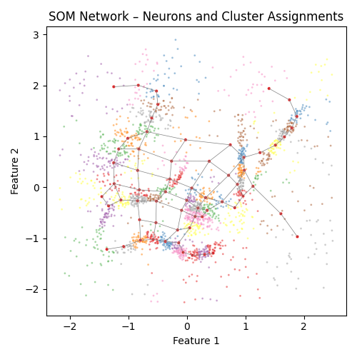
Network Visualization

Input data colored by cluster assignment; gray lines show neuron connections.

edges = list(som.som_.edges)
weights = som.weights_

fig, ax = plt.subplots(figsize=(5, 5))
for edge in edges:
    ax.plot(
        [
            som.som_.nodes().data()[edge[0]]["weight"][0],
            som.som_.nodes().data()[edge[1]]["weight"][0],
        ],
        [
            som.som_.nodes().data()[edge[0]]["weight"][1],
            som.som_.nodes().data()[edge[1]]["weight"][1],
        ],
        color="gray",
        linewidth=0.5,
    )
sns.scatterplot(
    ax=ax,
    x=data[:, 0],
    y=data[:, 1],
    s=4,
    alpha=0.5,
    hue=som.predict(data),
    palette="Set1",
    legend=False,
)
sns.scatterplot(
    ax=ax,
    x=weights[:, 0],
    y=weights[:, 1],
    hue=[1] * len(som.neurons_),
    palette="Set1",
    s=10,
    legend=False,
)
ax.set_title("SOM Network – Neurons and Cluster Assignments")
ax.set_xlabel("Feature 1")
ax.set_ylabel("Feature 2")
plt.tight_layout()
plt.show()

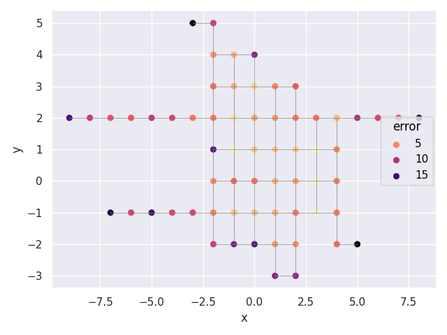
Quantization Error per Neuron

Each neuron colored by mean quantization error — higher error (darker) indicates regions where data density is not well represented.

som.plot(color="error").show()

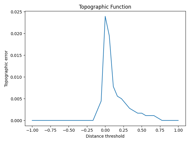
Topographic Function

Topographic error as a function of distance threshold. Lower values indicate better topology preservation.

te = som.topographic_function(data)
fig, ax = plt.subplots()
ax.plot(te[1], te[0])
ax.set_xlabel("Distance threshold")
ax.set_ylabel("Topographic error")
ax.set_title("Topographic Function")
plt.tight_layout()
plt.show()